Interpreting FOS results with fault interfaces in FLAC3D

Hi everyone,
I am currently running a model of an open pit with faults using FLAC3D v7. The geological units were imported as DXF files, while the faults were added as planar structures via Griddle and defined as interfaces in the model:


; ---------------- Fault properties ------------------

zone interface name 'F1' node prop stiffness-normal 0.559e9 stiffness-shear 0.224e9 fric 35 coh 0.22e6 ten 0.02e6
zone interface name 'F2' node prop stiffness-normal 0.559e9 stiffness-shear 0.224e9 fric 35 coh 0.22e6 ten 0.02e6
zone interface name 'F3' node prop stiffness-normal 6.785e9 stiffness-shear 2.714e9 fric 36 coh 0.25e6 ten 0.02e6

The outer rock mass is modeled using the Mohr-Coulomb (MC) criterion, while the pit area uses Hoek-Brown (HB). Since the host rock is expected to be anisotropic, I’ve applied the Ubiquitous-Joint model only in a close area to the pit (not all model to save some calculation time).
To simulate a disturbance around the pit during excavation stage, the parameters are reduced using the Disturbance factor of 0,7.
I run two models:

  • Test01: FOS calculation without considering faults (strength reduction applied only to rock mass).
  • Test02: FOS calculation considering faults (strength reduction applied to both rock mass and fault parameters).
; ---------------- computed models ------------------
model rest 'Test01'
model factor-of-safety convergence 1 filename 'Test01_Conv1_FOS_V00'

model rest 'Test01'
model factor-of-safety convergence 1 filename 'Test02_Conv1_Fault_FOS_V00' interface include 'friction' include 'cohesion'

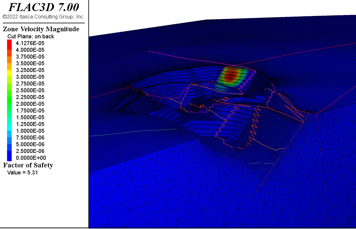
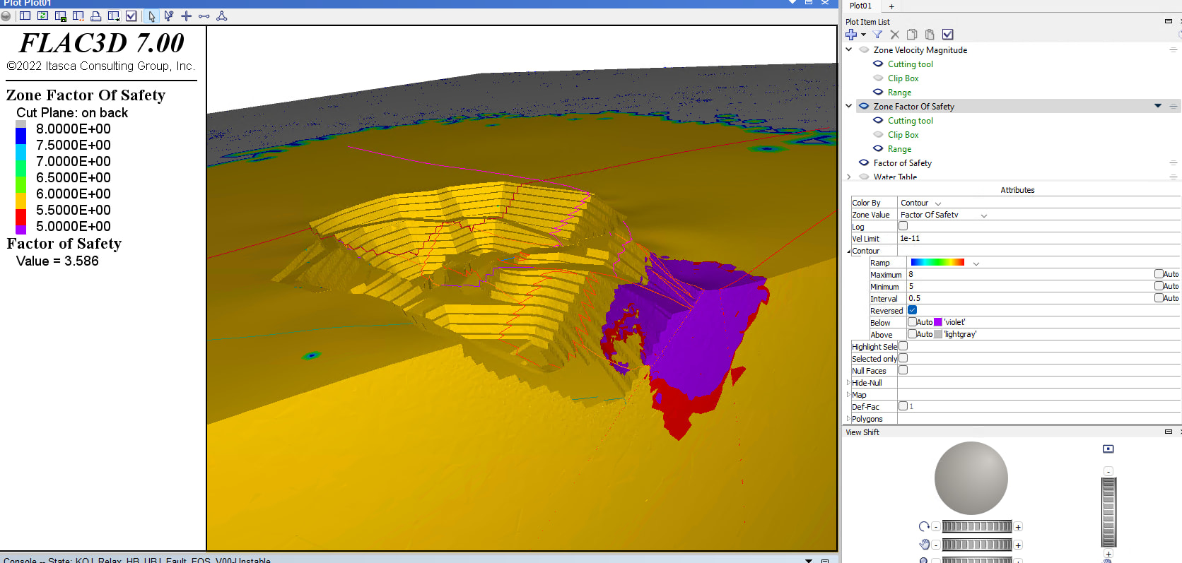
Both plots are from the Unstable .SAV results. For Test02, the velocity limits had to be set to 1e-11 to visualize changes in the FOS plot.
Why does reducing fault strength cause such a large increase in localized velocity compared to leaving faults constant? Which approach is generally considered more representative for open pit FOS analysis?

Any guidance or suggestions would be greatly appreciated.
Cheers,
Luca

as i can see, yout FOS are very high… what are the properties of rock mass and faults? check that the properties are been properly reduced by the command.

Always check the results with displacement histories (if it is unstable, the behaviour must be accelerated)

Vel of 1e-11 seems to me very low…

Your model is with a very high FOS > 5.0. For such a high FOS, trying to plot FOS contour with a very low velocity limit is practically unnecessary.

Hello and Happy New Year!
Thank you for your help in my previous thread! @msepu, I checked the property plots and they look correct. The Ubiquitous Joint and Mohr‑Coulomb parameters are reduced by the FOS procedure at failure, and Hoek‑Brown shows the expected non‑linear behavior.

Since then, I updated the model:

  • refreshed fault interface properties and ubiquitous joint parameters,
  • set a conservative phreatic surface ~1 m behind the pit wall,
  • and skipped convergence criterion #1, which was too conservative near faults close to the face.
model rest 'Model_00'
;------------- zone properties (Pa) TEST01 - Interface vary by Proxy ------------------

zone cmodel assign mohr-coulomb
; LITHO1 domain for all the zone MC paramters
zone property bulk 31.2e9 shear 18.7e9 dilation 6 cohesion 3.26e6 friction 51 tension 0.65e6 density 2785

zone cmodel assign hoek-brown range group 'LITHO2' or 'LITHO3' or 'LITHO4' or 'LITHO5'
zone property bulk 28.77e9 shear 17.26e9 density 2875 constant-dilation 6 constant-a 0.503 constant-mb 2.959 constant-s 0.012 constant-sci 95e6 tension 0.38e6 range group 'LITHO2'
zone property bulk 20.45e9 shear 12.27e9 density 2930 constant-dilation 5 constant-a 0.503 constant-mb 2.152 constant-s 0.012 constant-sci 65e6 tension 0.35e6 range group 'LITHO3'
zone property bulk 23.92e9 shear 14.35e9 density 2950 constant-dilation 5 constant-a 0.503 constant-mb 2.348 constant-s 0.012 constant-sci 66e6 tension 0.33e6 range group 'LITHO4'
zone property bulk 35.8e9 shear 21.48e9 density 2955 constant-dilation 6 constant-a 0.502 constant-mb 3.986 constant-s 0.02 constant-sci 150e6 tension 0.77e6 range group 'LITHO5'

zone cmodel assign ubiquitous-joint range group 'LITHO1_UBJ' or 'LITHO6_UBJ'
zone property bulk 26.1e9 shear 15.7e9 dilation 6 cohesion 3.47e6 friction 49 tension 0.77e6 density 2930 dip 43 dip-dir 338 joint-cohesion 0.01e6 joint-friction 26 joint-tension 0e6 joint-dilation 0 ran group 'LITHO6_UBJ'
zone property bulk 31.2e9 shear 18.7e9 dilation 6 cohesion 3.26e6 friction 51 tension 0.65e6 density 2785 dip 43 dip-dir 338 joint-cohesion 0.01e6 joint-friction 26 joint-tension 0e6 joint-dilation 0 ran group 'LITHO1_UBJ'


; ---------------- Fault properties ------------------
; assumptions

zone interface name 'F1' node prop stiffness-normal 1e9 stiffness-shear 0.5e9 fric 15 coh 0.02e6
zone interface name 'F1' node prop stiffness-normal 0.3e9 stiffness-shear 0.15e9 fric 15 coh 0.02e6 range geometry-distance 'KOJ_Aug25_Pit' gap 100 extent

zone interface name 'F2' node prop stiffness-normal 2e9 stiffness-shear 1e9 fric 19 coh 0.02e6
zone interface name 'F2' node prop stiffness-normal 1e9 stiffness-shear 0.5e9 fric 19 coh 0.02e6 range geometry-distance 'KOJ_Aug25_Pit' gap 100 extent

zone interface name 'F3' node prop stiffness-normal 6e9 stiffness-shear 4e9 fric 28 coh 0.06e6
zone interface name 'F3' node prop stiffness-normal 3e9 stiffness-shear 2e9 fric 28 coh 0.06e6 range geometry-distance 'KOJ_Aug25_Pit' gap 100 extent

zone interface name 'F4' node prop stiffness-normal 2e9 stiffness-shear 1e9 fric 18 coh 0.02e6
zone interface name 'F4' node prop stiffness-normal 1e9 stiffness-shear 0.5e9 fric 18 coh 0.02e6 range geometry-distance 'KOJ_Aug25_Pit' gap 100 extent

zone interface name 'Shear_Contact' node prop stiffness-normal 0.3e9 stiffness-shear 0.2e9 fric 18 coh 0.01e6

;---------------- Initial stress ----------------
model gravity 0,0,-9.81
zone initialize-stresses
zone interface node ini-stress

model solve ratio 1e-6
model save 'InSitu_HB_Base_FTStiffnessByProxy_T02'

zone gridpoint initialize displacement 0 0 0
zone gridpoint initialize velocity 0 0 0
zone initialize state 0

zone property bulk 11.1e9 shear 6.66e9 density 2875 constant-dilation 5 constant-a 0.503 constant-mb 1.371 constant-s 0.003 constant-sci 95e6 tension 0.21e6 range group 'LITHO2' and 'DFactor=D07'
zone property bulk 8.58e9 shear 4.66e9 density 2930 constant-dilation 5 constant-a 0.503 constant-mb 0.997 constant-s 0.003 constant-sci 65e6 tension 0.2e6 range group 'LITHO3' and 'DFactor=D07'
zone property bulk 10.03e9 shear 5.45e9 density 2950 constant-dilation 5 constant-a 0.503 constant-mb 1.088 constant-s 0.003 constant-sci 66e6 tension 0.18e6 range group 'LITHO4' and 'DFactor=D07'
zone property bulk 37.6e9 shear 8.06e9 density 2955 constant-dilation 6 constant-a 0.502 constant-mb 2.033 constant-s 0.006 constant-sci 150e6 tension 0.46e6 range group 'LITHO5' and 'DFactor=D07'

zone property bulk 13.7e9 shear 6.3e9 dilation 6 cohesion 2.07e6 friction 46 tension 0.46e6 density 2930 dip 43 dip-dir 338 joint-cohesion 0e6 joint-friction 26 joint-tension 0e6 joint-dilation 0 ran group 'LITHO6_UBJ' and 'DFactor=D07'
zone property bulk 21.8e9 shear 7.3e9 dilation 6 cohesion 1.95e6 friction 48 tension 0.39e6 density 2785 dip 43 dip-dir 338 joint-cohesion 0e6 joint-friction 26 joint-tension 0e6 joint-dilation 0 ran group 'LITHO1_UBJ' and 'DFactor=D07'

model history name='conv' mechanical convergence
model history name='UM' mech unbalanced-maximum

zone relax excavate range group 'Model=Pit'
model solve ratio 1e-6
model save 'HB_UBJ_Base_FTStiffnessByProxy_T02'

;============================
; water parameters
;============================
geometry import 'geom_clips\water\Water_1mBelowPit.dxf'
zone water density 1000
zone water set 'Water_1mBelowPit'

model solve ratio 1e-6
model save 'HB_UBJ_Water1m_Base_FTStiffnessByProxy_T02'

;model factor-of-safety filename 'FOS_Water1m_Base_FTStiffnessByProxy_T03'; interface include 'friction' include 'cohesion'
model factor-of-safety filename 'FOS_Water1m_Base_FTStiffnessByProxy_T04' bracket 0.25 2.0 bracket-limit 0.05; interface include 'friction' include 'cohesion'

Baseline result:

  • Global stability (SSR): the model stays stable up to the specified limit (global FoS acceptable).
  • Local behavior: a zone of reduced stability is observed along the North‑East wall, near fault F1 and in areas where different geological units are exposed.
    I would appreciate your views on three points:
  1. Fault stiffness changing with depth (soft buffer near the pit wall)
    In the baseline, I use lower kn/ks within ~100 m of the wall (to represent damage and stress relief), and increase stiffness with depth beyond 100 m.
    Is this simplification reasonable for SSR in open pits?
    Any suggested ks/kn ratios or preferred functions that you find useful?

  2. Include fault shear strength in SSR reduction?
    When I run model factor-of-safety, should I include fault/interface cohesion and friction (joint-c, joint-φ) in the reduction together with rock‑mass c and φ?
    My understanding: Yes—if the mechanism can slip along the fault, then fault c and tanφ should also be reduced, otherwise global FoS may be overestimated.
    Does this match your practice? Any risk should i consider when linking interface properties to the SRF?

  3. Interpret global SSR FoS vs local FoS with a velocity limit
    I plot a FoS heatmap with a velocity limit (e.g., 1e‑5) to focus on active zones. This shows local FoS < 0.5 in the NE wall, while the global SSR says the slope is stable (e.g., SRF > 2).

Plot by set velocity limits to 1e-5

My interpretation: global FoS (SSR) = system stability for design, and local FoS = a local yield indicator (where strain begins).
Is this a correct way to communicate results (globally stable, but localized risk bands)? Do you recommend different velocity thresholds (e.g., 1e‑4 or 1e‑3) for cleaner diagnostic plots? Is there a way to show contour lines at specific FoS values (like 1.2 or 1.3) in the plot?
Any examples, workflows, or parameter ranges would be very helpful.

Hello Luca,
There is a Paper of D. Martin (if i’m not wrong) talking about the kn/ks ratios, i encourage you to take a look at it.

Yes, you should include a reduction on faults properties too

Theres is no a “magical” value of velocity to interpret stable/unstable mechanisms, you must include displacement histories, strain, plasticity. The velocity limit you use, must match with those other indicators.

Mmmm i do not know if is there anyway to plot at specific FOS values…. probably modifying the contour scale?

Regards,

Hi,
Thanks a lot @msepu. Yes, I think you are referring to the MÜLLER LECTURE he presented in 2023. I have been taking that into account when estimating the stiffness.

Regarding the velocity limits, I am referring to Chapter 10 Numerical Analysis by Lorig & Varona in Rock Slope Engineering book, where they write:

“…velocities below 1e‑6 indicate stability in FLAC and FLAC3D; conversely, velocities above 1e‑5 indicate instability.”

I understand that there is no strict “magical” limit. When I interpret result I always check the displacement, maximum shear strain increment, and the stress plots. Then I interpret the results and the possible failure mechanism.

My question about the FoS heatmap is because clients increasingly want a simple, visual FoS plot rather than multiple separate plots of displacement/stress/strain. I am trying to understand the best way to display a FoS heatmap in FLAC3D without writing a FISH code.

I run the model including the interfaces. The figure below shows the FOS for the Unstable file. The global FOS is around 7 but I reduce the velocity limit to 1e-5, several local FOS < 0.5 area appear.


Lowering the velocity limit helps me highlight potentially critical zones for further review, even though the overall slope is clearly stable.

For example, based on the shear strain increment (cross‑section location marked in the plan view), the failure of the lower benches might trigger toward a deep‑seated circular mechanism on the NE wall, while the SE wall, where foliation dominates, shows a more planar‑type response. However, under the applied conditions (FoS ≈ 7), these failures are highly unlikely.
Am I misinterpreting these results? I want to be sure I am understanding the local “instabilities” correctly when the overall model is extremely stable (The plots shows the Unstable .sav file)

Finally, I would like to perform a sensitivity test for pore-pressure without a full hydro-mechanical model. I have already imported and run the model using a phreatic surface. I checked the documentation and examples but I could not find a clear workflow for applying pore pressure based on an imported DXF surface.

  • Is it possible to assign pore pressure directly from an imported DXF surface
  • Or is it better to use the built‑in zone set water ... commands and simply modify the geometry of the DXF surface instead?

Thanks again for your help!